

On the earth of actual property, quite a few components affect property costs. The financial system, market demand, location, and even the 12 months a property is bought can play vital roles. The years 2007 to 2009 marked a tumultuous time for the US housing market. This era, also known as the Nice Recession, noticed a drastic decline in residence values, a surge in foreclosures, and widespread monetary market turmoil. The influence of the recession on housing costs was profound, with many owners discovering themselves in properties that had been value lower than their mortgages. The ripple impact of this downturn was felt throughout the nation, with some areas experiencing sharper declines and slower recoveries than others.
Given this backdrop, it’s significantly intriguing to investigate housing information from Ames, Iowa, because the dataset spans from 2006 to 2010, encapsulating the peak and aftermath of the Nice Recession. Does the 12 months of sale, amidst such financial volatility, affect the gross sales worth in Ames? On this put up, you’ll delve deep into the Ames Housing dataset to discover this question utilizing Exploratory Knowledge Evaluation (EDA) and two statistical exams: ANOVA and the Kruskal-Wallis Check.
Let’s get began.
Leveraging ANOVA and Kruskal-Wallis Assessments to Analyze the Impression of the Nice Recession on Housing PricesPhoto by Sharissa Johnson. Some rights reserved.
Overview
This put up is split into three elements; they’re:
EDA: Visible Insights
Assessing Variability in Gross sales Costs Throughout Years Utilizing ANOVA
Kruskal-Wallis Check: A Non-Parametric Various to ANOVA
EDA: Visible Insights
To start, let’s load the Ames Housing dataset and evaluate totally different years of sale towards the dependent variable: the gross sales worth.
# Importing the important libraries
import pandas as pd
import seaborn as sns
import matplotlib.pyplot as plt
# Load the dataset
Ames = pd.read_csv(‘Ames.csv’)
# Convert ‘YrSold’ to a categorical variable
Ames[‘YrSold’] = Ames[‘YrSold’].astype(‘class’)
plt.determine(figsize=(10, 6))
sns.boxplot(x=Ames[‘YrSold’], y=Ames[‘SalePrice’], hue=Ames[‘YrSold’])
plt.title(‘Boxplot of Gross sales Costs by Yr’, fontsize=18)
plt.xlabel(‘Yr Offered’, fontsize=15)
plt.ylabel(‘Gross sales Value (US$)’, fontsize=15)
plt.legend(”)
plt.present()
1
2
3
4
5
6
7
8
9
10
11
12
13
14
15
16
17
18
# Importing the important libraries
import pandas as pd
import seaborn as sns
import matplotlib.pyplot as plt
# Load the dataset
Ames = pd.read_csv(‘Ames.csv’)
# Convert ‘YrSold’ to a categorical variable
Ames[‘YrSold’] = Ames[‘YrSold’].astype(‘class’)
plt.determine(figsize=(10, 6))
sns.boxplot(x=Ames[‘YrSold’], y=Ames[‘SalePrice’], hue=Ames[‘YrSold’])
plt.title(‘Boxplot of Gross sales Costs by Yr’, fontsize=18)
plt.xlabel(‘Yr Offered’, fontsize=15)
plt.ylabel(‘Gross sales Value (US$)’, fontsize=15)
plt.legend(”)
plt.present()
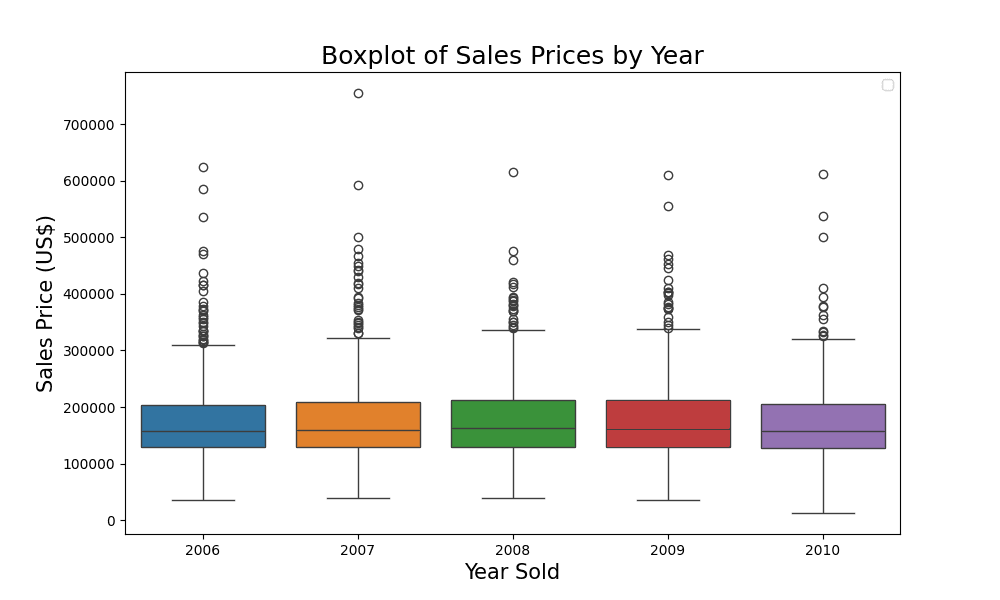
Evaluating the pattern of gross sales costs
From the boxplot, you may observe that the gross sales costs had been fairly constant throughout totally different years as a result of every year seems alike. Let’s take a better look utilizing the groupby perform in pandas.
# Calculating imply and median gross sales worth by 12 months
summary_table = Ames.groupby(‘YrSold’)[‘SalePrice’].agg([‘mean’, ‘median’])
# Rounding the values for higher presentation
summary_table = summary_table.spherical(2)
print(summary_table)
# Calculating imply and median gross sales worth by 12 months
summary_table = Ames.groupby(‘YrSold’)[‘SalePrice’].agg([‘mean’, ‘median’])
# Rounding the values for higher presentation
summary_table = summary_table.spherical(2)
print(summary_table)
The output is:
imply median
YrSold
2006 176615.62 157000.0
2007 179045.08 159000.0
2008 178170.02 162700.0
2009 180387.64 162000.0
2010 173971.67 157900.0
imply median
YrSold
2006 176615.62 157000.0
2007 179045.08 159000.0
2008 178170.02 162700.0
2009 180387.64 162000.0
2010 173971.67 157900.0
From the desk, you may make the next observations:
The imply gross sales worth was the best in 2009 at roughly $180,388, whereas it was the bottom in 2010 at round $173,972.
The median gross sales worth was the best in 2008 at $162,700 and the bottom in 2006 at $157,000.
Though the imply and median gross sales costs are shut in worth for every year, there are slight variations. This means that whereas there is perhaps some outliers influencing the imply, they don’t seem to be extraordinarily skewed.
Over the 5 years, there doesn’t appear to be a constant upward or downward pattern in gross sales costs, which is attention-grabbing given the bigger financial context (the Nice Recession) throughout this era.
This desk, mixed with the boxplot, provides a complete view of the distribution and central tendency of gross sales costs throughout the years. It units the stage for deeper statistical evaluation to find out if the noticed variations (or lack thereof) are statistically vital.
Kick-start your mission with my e-book The Newbie’s Information to Knowledge Science. It offers self-study tutorials with working code.
Assessing Variability in Gross sales Costs Throughout Years Utilizing ANOVA
ANOVA (Evaluation of Variance) helps us take a look at if there are any statistically vital variations between the technique of three or extra unbiased teams. Its null speculation is that the technique of all teams are equal. This may be thought of as a model of t-test to help greater than two teams. It makes use of the F-test statistic to test if the variance ($sigma^2$) is totally different inside every group in comparison with throughout all teams.
The speculation setup is:
$H_0$: The technique of gross sales worth for all years are equal.
$H_1$: Not less than one 12 months has a special imply gross sales worth.
You may run your take a look at utilizing the scipy.stats library as follows:
# Import a further library
import scipy.stats as stats
# Carry out the ANOVA
f_value, p_value = stats.f_oneway(*[Ames[‘SalePrice’][Ames[‘YrSold’] == 12 months]
for 12 months in Ames[‘YrSold’].distinctive()])
print(f_value, p_value)
# Import a further library
import scipy.stats as stats
# Carry out the ANOVA
f_value, p_value = stats.f_oneway(*[Ames[‘SalePrice’][Ames[‘YrSold’] == 12 months]
for 12 months in Ames[‘YrSold’].distinctive()])
print(f_value, p_value)
The 2 values are:
0.4478735462379817 0.774024927554816
0.4478735462379817 0.774024927554816
The outcomes of the ANOVA take a look at are:
F-value: 0.4479
p-value: 0.7740
Given the excessive p-value (higher than a standard significance degree of 0.05), you can not reject the null speculation ($H_0$). This means that there are not any statistically vital variations between the technique of gross sales worth for the totally different years current within the dataset.
Whereas your ANOVA outcomes present insights into the equality of means throughout totally different years, it’s important to make sure that the assumptions underlying the take a look at have been met. Let’s delve into verifying the three assumptions of ANOVA exams to validate your findings.
Assumption 1: Independence of Observations. Since every remark (home sale) is unbiased of one other, this assumption is met.
Assumption 2: Normality of the Residuals. For ANOVA to be legitimate, the residuals from the mannequin ought to roughly observe a traditional distribution since that is the mannequin behind F-test. You may test this each visually and statistically.
Visible evaluation will be executed utilizing a QQ plot:
# Import a further library
import statsmodels.api as sm
# Match an unusual least squares mannequin and get residuals
mannequin = sm.OLS(Ames[‘SalePrice’], Ames[‘YrSold’].astype(‘int’)).match()
residuals = mannequin.resid
# Plot QQ plot
sm.qqplot(residuals, line=”s”)
plt.title(‘Normality Evaluation of Residuals by way of QQ Plot’, fontsize=18)
plt.xlabel(‘Theoretical Quantiles’, fontsize=15)
plt.ylabel(‘Pattern Residual Quantiles’, fontsize=15)
plt.grid(True, which=”each”, linestyle=”–“, linewidth=0.5)
plt.present()
# Import a further library
import statsmodels.api as sm
# Match an unusual least squares mannequin and get residuals
mannequin = sm.OLS(Ames[‘SalePrice’], Ames[‘YrSold’].astype(‘int’)).match()
residuals = mannequin.resid
# Plot QQ plot
sm.qqplot(residuals, line=‘s’)
plt.title(‘Normality Evaluation of Residuals by way of QQ Plot’, fontsize=18)
plt.xlabel(‘Theoretical Quantiles’, fontsize=15)
plt.ylabel(‘Pattern Residual Quantiles’, fontsize=15)
plt.grid(True, which=‘each’, linestyle=‘–‘, linewidth=0.5)
plt.present()
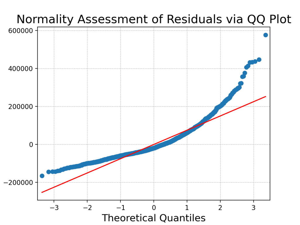
The QQ Plot offered above serves as a beneficial visible device to evaluate the normality of your dataset’s residuals, providing insights into how nicely the noticed information aligns with the theoretical expectations of a traditional distribution. On this plot, every level represents a pair of quantiles: one from the residuals of your information and the opposite from the usual regular distribution. Ideally, in case your information completely adopted a traditional distribution, all of the factors on the QQ Plot would fall exactly alongside the pink 45-degree reference line. The plot illustrates deviations from the 45-degree reference line, suggesting potential deviations from normality.
Statistical evaluation will be executed utilizing the Shapiro-Wilk Check, which offers a proper methodology to check for normality. The null speculation of the take a look at is that the info follows a traditional distribution. This take a look at additionally out there in SciPy:
#Import shapiro from scipy.stats bundle
from scipy.stats import shapiro
# Shapiro-Wilk Check
shapiro_stat, shapiro_p = shapiro(residuals)
print(f”Shapiro-Wilk Check Statistic: {shapiro_stat}nP-value: {shapiro_p}”)
#Import shapiro from scipy.stats bundle
from scipy.stats import shapiro
# Shapiro-Wilk Check
shapiro_stat, shapiro_p = shapiro(residuals)
print(f“Shapiro-Wilk Check Statistic: {shapiro_stat}nP-value: {shapiro_p}”)
The output is:
Shapiro-Wilk Check Statistic: 0.8774482011795044
P-value: 4.273399796804962e-41
Shapiro-Wilk Check Statistic: 0.8774482011795044
P-value: 4.273399796804962e-41
A low p-value (sometimes p < 0.05) suggests rejecting the null speculation, indicating that the residuals don’t observe a traditional distribution. This means a violation of the second assumption of ANOVA, which requires that the residuals be usually distributed. Each the QQ plot and the Shapiro-Wilk take a look at converge on the identical conclusion: the residuals don’t strictly adhere to a traditional distribution. Therefore, the results of the ANOVA is probably not legitimate.
Assumption 3: Homogeneity of Variances. The variances of the teams (years) must be roughly equal. This occurs to be the null speculation of Levene’s take a look at. Therefore you need to use it to confirm:
# Verify for equal variances utilizing Levene’s take a look at
levene_stat, levene_p = stats.levene(*[Ames[‘SalePrice’][Ames[‘YrSold’] == 12 months]
for 12 months in Ames[‘YrSold’].distinctive()])
print(f”Levene’s Check Statistic: {levene_stat}nP-value: {levene_p}”)
# Verify for equal variances utilizing Levene’s take a look at
levene_stat, levene_p = stats.levene(*[Ames[‘SalePrice’][Ames[‘YrSold’] == 12 months]
for 12 months in Ames[‘YrSold’].distinctive()])
print(f“Levene’s Check Statistic: {levene_stat}nP-value: {levene_p}”)
The output is:
Levene’s Check Statistic: 0.2514412478357097
P-value: 0.9088910499612235
Levene’s Check Statistic: 0.2514412478357097
P-value: 0.9088910499612235
Given the excessive p-value of 0.909 from Levene’s take a look at, you can not reject the null speculation, indicating that the variances of gross sales costs throughout totally different years are statistically homogeneous, satisfying the third key assumption for ANOVA.
Placing all collectively, the next code runs the ANOVA take a look at and verifies the three assumptions:
# Importing the important libraries
import pandas as pd
import scipy.stats as stats
import matplotlib.pyplot as plt
import statsmodels.api as sm
from scipy.stats import shapiro
# Load the dataset
Ames = pd.read_csv(‘Ames.csv’)
# Carry out the ANOVA
f_value, p_value = stats.f_oneway(*[Ames[‘SalePrice’][Ames[‘YrSold’] == 12 months]
for 12 months in Ames[‘YrSold’].distinctive()])
print(“F-value:”, f_value)
print(“p-value:”, p_value)
# Match an unusual least squares mannequin and get residuals
mannequin = sm.OLS(Ames[‘SalePrice’], Ames[‘YrSold’].astype(‘int’)).match()
residuals = mannequin.resid
# Plot QQ plot
sm.qqplot(residuals, line=”s”)
plt.title(‘Normality Evaluation of Residuals by way of QQ Plot’, fontsize=18)
plt.xlabel(‘Theoretical Quantiles’, fontsize=15)
plt.ylabel(‘Pattern Residual Quantiles’, fontsize=15)
plt.grid(True, which=”each”, linestyle=”–“, linewidth=0.5)
plt.present()
# Shapiro-Wilk Check
shapiro_stat, shapiro_p = shapiro(residuals)
print(f”Shapiro-Wilk Check Statistic: {shapiro_stat}nP-value: {shapiro_p}”)
# Verify for equal variances utilizing Levene’s take a look at
levene_stat, levene_p = stats.levene(*[Ames[‘SalePrice’][Ames[‘YrSold’] == 12 months]
for 12 months in Ames[‘YrSold’].distinctive()])
print(f”Levene’s Check Statistic: {levene_stat}nP-value: {levene_p}”)
1
2
3
4
5
6
7
8
9
10
11
12
13
14
15
16
17
18
19
20
21
22
23
24
25
26
27
28
29
30
31
32
33
34
35
36
37
# Importing the important libraries
import pandas as pd
import scipy.stats as stats
import matplotlib.pyplot as plt
import statsmodels.api as sm
from scipy.stats import shapiro
# Load the dataset
Ames = pd.read_csv(‘Ames.csv’)
# Carry out the ANOVA
f_value, p_value = stats.f_oneway(*[Ames[‘SalePrice’][Ames[‘YrSold’] == 12 months]
for 12 months in Ames[‘YrSold’].distinctive()])
print(“F-value:”, f_value)
print(“p-value:”, p_value)
# Match an unusual least squares mannequin and get residuals
mannequin = sm.OLS(Ames[‘SalePrice’], Ames[‘YrSold’].astype(‘int’)).match()
residuals = mannequin.resid
# Plot QQ plot
sm.qqplot(residuals, line=‘s’)
plt.title(‘Normality Evaluation of Residuals by way of QQ Plot’, fontsize=18)
plt.xlabel(‘Theoretical Quantiles’, fontsize=15)
plt.ylabel(‘Pattern Residual Quantiles’, fontsize=15)
plt.grid(True, which=‘each’, linestyle=‘–‘, linewidth=0.5)
plt.present()
# Shapiro-Wilk Check
shapiro_stat, shapiro_p = shapiro(residuals)
print(f“Shapiro-Wilk Check Statistic: {shapiro_stat}nP-value: {shapiro_p}”)
# Verify for equal variances utilizing Levene’s take a look at
levene_stat, levene_p = stats.levene(*[Ames[‘SalePrice’][Ames[‘YrSold’] == 12 months]
for 12 months in Ames[‘YrSold’].distinctive()])
print(f“Levene’s Check Statistic: {levene_stat}nP-value: {levene_p}”)
Kruskal-Wallis Check: A Non-Parametric Various to ANOVA
The Kruskal-Wallis take a look at is a non-parametric methodology used to check the median values of three or extra unbiased teams, making it an appropriate various to the one-way ANOVA (particularly when assumptions of ANOVA usually are not met).
Non-parametric statistics are a category of statistical strategies that don’t make express assumptions in regards to the underlying distribution of the info. In distinction to parametric exams, which assume a particular distribution (e.g., regular distribution in assumption 2 above), non-parametric exams are extra versatile and will be utilized to information that won’t meet the stringent assumptions of parametric strategies. Non-parametric exams are significantly helpful when coping with ordinal or nominal information, in addition to information which may exhibit skewness or heavy tails. These exams concentrate on the order or rank of values quite than the precise values themselves. Non-parametric exams, together with the Kruskal-Wallis take a look at, supply a versatile and distribution-free strategy to statistical evaluation, making them appropriate for a variety of information varieties and conditions.
The speculation setup underneath Kruskal-Wallis take a look at is:
$H_0$: The distributions of the gross sales worth for all years are equivalent.
$H_1$: Not less than one 12 months has a special distribution of gross sales worth.
You may run Kruskal-Wallis take a look at utilizing SciPy, as follows:
# Carry out the Kruskal-Wallis H-test
H_statistic, kruskal_p_value = stats.kruskal(*[Ames[‘SalePrice’][Ames[‘YrSold’] == 12 months]
for 12 months in Ames[‘YrSold’].distinctive()])
print(H_statistic, kruskal_p_value)
# Carry out the Kruskal-Wallis H-test
H_statistic, kruskal_p_value = stats.kruskal(*[Ames[‘SalePrice’][Ames[‘YrSold’] == 12 months]
for 12 months in Ames[‘YrSold’].distinctive()])
print(H_statistic, kruskal_p_value)
The output is:
2.1330989438609236 0.7112941815590765
2.1330989438609236 0.7112941815590765
The outcomes of the Kruskal-Wallis take a look at are:
H-Statistic: 2.133
p-value: 0.7113
Notice: The Kruskal-Wallis take a look at doesn’t particularly take a look at for variations in means (like ANOVA does), however quite for variations in distributions. This will embrace variations in medians, shapes, and spreads.
Given the excessive p-value (higher than a standard significance degree of 0.05), you can not reject the null speculation. This means that there are not any statistically vital variations within the median gross sales costs for the totally different years current within the dataset when utilizing the Kruskal-Wallis take a look at. Let’s delve into verifying the three assumptions of the Kruskal-Wallis take a look at to validate your findings.
Assumption 1: Independence of Observations. This stays the identical as for ANOVA; every remark is unbiased of one other.
Assumption 2: The Response Variable Must be Ordinal, Interval, or Ratio. The gross sales worth is a ratio variable, so this assumption is met.
Assumption 3: The Distributions of the Response Variable Must be the Similar for All Teams. This may be validated utilizing each visible and numerical strategies.
# Plot histograms of Gross sales Value for every year
fig, axes = plt.subplots(nrows=5, ncols=1, figsize=(12, 8), sharex=True)
for idx, 12 months in enumerate(sorted(Ames[‘YrSold’].distinctive())):
sns.histplot(Ames[Ames[‘YrSold’] == 12 months][‘SalePrice’], kde=True, ax=axes[idx], coloration=”skyblue”)
axes[idx].set_title(f’Distribution of Gross sales Costs for Yr {12 months}’, fontsize=16)
axes[idx].set_ylabel(‘Frequency’, fontsize=14)
if idx == 4:
axes[idx].set_xlabel(‘Gross sales Value’, fontsize=15)
else:
axes[idx].set_xlabel(”)
plt.tight_layout()
plt.present()
# Plot histograms of Gross sales Value for every year
fig, axes = plt.subplots(nrows=5, ncols=1, figsize=(12, 8), sharex=True)
for idx, 12 months in enumerate(sorted(Ames[‘YrSold’].distinctive())):
sns.histplot(Ames[Ames[‘YrSold’] == 12 months][‘SalePrice’], kde=True, ax=axes[idx], coloration=‘skyblue’)
axes[idx].set_title(f‘Distribution of Gross sales Costs for Yr {12 months}’, fontsize=16)
axes[idx].set_ylabel(‘Frequency’, fontsize=14)
if idx == 4:
axes[idx].set_xlabel(‘Gross sales Value’, fontsize=15)
else:
axes[idx].set_xlabel(”)
plt.tight_layout()
plt.present()
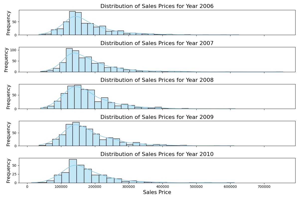
Distribution of gross sales costs of various years
The stacked histograms point out constant distributions of gross sales costs throughout the years, with every year displaying an identical vary and peak regardless of slight variations in frequency.
Moreover, you may conduct pairwise Kolmogorov-Smirnov exams, which is a non-parametric take a look at to check the similarity of two likelihood distributions. It’s out there in SciPy. You should utilize the model that the null speculation is the 2 distributions equal, and the choice speculation isn’t equal:
# Run KS Check from scipy.stats
from scipy.stats import ks_2samp
outcomes = {}
for i, year1 in enumerate(sorted(Ames[‘YrSold’].distinctive())):
for j, year2 in enumerate(sorted(Ames[‘YrSold’].distinctive())):
if i < j:
ks_stat, ks_p = ks_2samp(Ames[Ames[‘YrSold’] == year1][‘SalePrice’],
Ames[Ames[‘YrSold’] == year2][‘SalePrice’])
outcomes[f”{year1} vs {year2}”] = (ks_stat, ks_p)
# Convert the outcomes right into a DataFrame for tabular illustration
ks_df = pd.DataFrame(outcomes).transpose()
ks_df.columns = [‘KS Statistic’, ‘P-value’]
ks_df.reset_index(inplace=True)
ks_df.rename(columns={‘index’: ‘Years In contrast’}, inplace=True)
print(ks_df)
1
2
3
4
5
6
7
8
9
10
11
12
13
14
15
16
17
# Run KS Check from scipy.stats
from scipy.stats import ks_2samp
outcomes = {}
for i, year1 in enumerate(sorted(Ames[‘YrSold’].distinctive())):
for j, year2 in enumerate(sorted(Ames[‘YrSold’].distinctive())):
if i < j:
ks_stat, ks_p = ks_2samp(Ames[Ames[‘YrSold’] == year1][‘SalePrice’],
Ames[Ames[‘YrSold’] == year2][‘SalePrice’])
outcomes[f“{year1} vs {year2}”] = (ks_stat, ks_p)
# Convert the outcomes right into a DataFrame for tabular illustration
ks_df = pd.DataFrame(outcomes).transpose()
ks_df.columns = [‘KS Statistic’, ‘P-value’]
ks_df.reset_index(inplace=True)
ks_df.rename(columns={‘index’: ‘Years In contrast’}, inplace=True)
print(ks_df)
This exhibits:
Years In contrast KS Statistic P-value
0 2006 vs 2007 0.038042 0.798028
1 2006 vs 2008 0.052802 0.421325
2 2006 vs 2009 0.062235 0.226623
3 2006 vs 2010 0.040006 0.896946
4 2007 vs 2008 0.039539 0.732841
5 2007 vs 2009 0.044231 0.586558
6 2007 vs 2010 0.051508 0.620135
7 2008 vs 2009 0.032488 0.908322
8 2008 vs 2010 0.052752 0.603031
9 2009 vs 2010 0.053236 0.586128
Years In contrast KS Statistic P–worth
0 2006 vs 2007 0.038042 0.798028
1 2006 vs 2008 0.052802 0.421325
2 2006 vs 2009 0.062235 0.226623
3 2006 vs 2010 0.040006 0.896946
4 2007 vs 2008 0.039539 0.732841
5 2007 vs 2009 0.044231 0.586558
6 2007 vs 2010 0.051508 0.620135
7 2008 vs 2009 0.032488 0.908322
8 2008 vs 2010 0.052752 0.603031
9 2009 vs 2010 0.053236 0.586128
Whereas we glad solely 2 out of the three assumptions for ANOVA, we’ve met all the mandatory standards for the Kruskal-Wallis take a look at. The pairwise Kolmogorov-Smirnov exams point out that the distributions of gross sales costs throughout totally different years are remarkably constant. Particularly, the excessive p-values (all higher than the frequent significance degree of 0.05) suggest that there isn’t sufficient proof to reject the speculation that the gross sales costs for every year come from the identical distribution. These findings fulfill the belief for the Kruskal-Wallis Check that the distributions of the response variable must be the identical for all teams. This underscores the steadiness within the gross sales worth distributions from 2006 to 2010 in Ames, Iowa, regardless of the broader financial context.
Additional Studying
On-line
Assets
Abstract
Within the multi-dimensional world of actual property, a number of components, together with the 12 months of sale, can doubtlessly affect property costs. The US housing market skilled appreciable turbulence throughout the Nice Recession between 2007 and 2009. The examine focuses on housing information from Ames, Iowa, spanning 2006 to 2010, aiming to find out if the 12 months of sale affected the gross sales worth, significantly throughout this tumultuous interval.
The evaluation employed each the ANOVA and Kruskal-Wallis exams to gauge variations in gross sales costs throughout totally different years. Whereas ANOVA’s findings had been instructive, not all its underlying assumptions had been glad, notably the normality of residuals. Conversely, the Kruskal-Wallis take a look at met all its standards, suggesting extra dependable insights. Subsequently, relying solely on the ANOVA may have been deceptive with out the corroborative perspective of the Kruskal-Wallis take a look at.
Each the one-way ANOVA and the Kruskal-Wallis take a look at yielded constant outcomes, indicating no statistically vital variations in gross sales costs throughout the totally different years. This consequence is especially fascinating given the turbulent financial backdrop from 2006 to 2010. The findings show that property costs in Ames had been very steady and influenced primarily by native situations.
Particularly, you realized:
The significance of validating the assumptions of statistical exams, as seen with the ANOVA’s residuals normality problem.
The importance and software of each parametric (ANOVA) and non-parametric (Kruskal-Wallis) exams in evaluating information distributions.
How native components can insulate property markets, like that of Ames, Iowa, from broader financial downturns, emphasizing the nuanced nature of actual property pricing.
Do you have got any questions? Please ask your questions within the feedback under, and I’ll do my finest to reply.
Get Began on The Newbie’s Information to Knowledge Science!
Study the mindset to develop into profitable in information science tasks
…utilizing solely minimal math and statistics, purchase your talent by way of quick examples in Python
Uncover how in my new E book:The Newbie’s Information to Knowledge Science
It offers self-study tutorials with all working code in Python to show you from a novice to an skilled. It exhibits you find out how to discover outliers, verify the normality of information, discover correlated options, deal with skewness, test hypotheses, and far more…all to help you in making a narrative from a dataset.
Kick-start your information science journey with hands-on workouts
See What’s Inside


")

")


")


