

In a earlier tutorial, we explored logistic regression as a easy however fashionable machine studying algorithm for binary classification applied within the OpenCV library.
Up to now, now we have seen how logistic regression could also be utilized to a customized two-class dataset now we have generated ourselves.
On this tutorial, you’ll find out how the usual logistic regression algorithm, inherently designed for binary classification, will be modified to cater to multi-class classification issues by making use of it to a picture classification process.
After finishing this tutorial, you’ll know:
A number of of crucial traits of the logistic regression algorithm.
How the logistic regression algorithm will be modified for multi-class classification issues.
Tips on how to apply logistic regression to the issue of picture classification.
Let’s get began.
Logistic Regression for Picture Classification Utilizing OpenCVPhoto by David Marcu, some rights reserved.
Tutorial Overview
This tutorial is split into three elements; they’re:
Recap of What Logistic Regression Is
Modifying Logistic Regression for Multi-Class Classification Issues
Making use of Logistic Regression to a Multi-Class Classification Downside
Recap of What Logistic Regression Is
In a earlier tutorial, we began exploring OpenCV’s implementation of the logistic regression algorithm. Up to now, now we have utilized it to a customized two-class dataset that now we have generated, consisting of two-dimensional factors gathered into two clusters.
Following Jason Brownlee’s tutorials on logistic regression, now we have additionally recapped the details about logistic regression. We have now seen that logistic regression is carefully associated to linear regression as a result of they each contain a linear mixture of options in producing a real-valued output. Nevertheless, logistic regression extends this course of by making use of the logistic (or sigmoid) perform. Therefore its identify. It’s to map the real-valued output right into a chance worth inside a variety [0, 1]. This chance worth is then categorised as belonging to the default class if it exceeds a threshold of 0.5; in any other case, it’s categorised as belonging to the non-default class. This makes logistic regression inherently a way for binary classification.
The logistic regression mannequin is represented by as many coefficients as options within the enter information, plus an additional bias worth. These coefficients and bias values are discovered throughout coaching utilizing gradient descent or most chance estimation (MLE) methods.
Modifying Logistic Regression for Multi-Class Classification Issues
As talked about within the earlier part, the usual logistic regression methodology caters solely to two-class issues by how the logistic perform and the following thresholding course of map the real-valued output of the linear mixture of options into both class 0 or class 1.
Therefore, catering for multi-class classification issues (or issues that contain greater than two courses) with logistic regression requires modification of the usual algorithm.
One method to realize this entails splitting the multi-class classification downside into a number of binary (or two-class) classification subproblems. The usual logistic regression methodology can then be utilized to every subproblem. That is how OpenCV implements multi-class logistic regression:
… Logistic Regression helps each binary and multi-class classifications (for multi-class it creates a a number of 2-class classifiers).
– Logistic Regression, OpenCV
A method of this sort is named the one-vs-one strategy, which entails coaching a separate binary classifier for every distinctive pair of courses within the dataset. Throughout prediction, every of those binary classifiers votes for one of many two courses on which it was educated, and the category that receives probably the most votes throughout all classifiers is taken to be the expected class.
There are different methods to realize multi-class classification with logistic regression, similar to via the one-vs-rest strategy. Chances are you’ll discover additional info in these tutorials [1, 2].
Making use of Logistic Regression to a Multi-Class Classification Downside
For this objective, we will be utilizing the digits dataset in OpenCV, though the code we are going to develop may additionally be utilized to different multi-class datasets.
Our first step is to load the OpenCV digits picture, divide it into its many sub-images that function handwritten digits from 0 to 9, and create their corresponding floor reality labels that may allow us to quantify the accuracy of the educated logistic regression mannequin later. For this explicit instance, we are going to allocate 80% of the dataset photographs to the coaching set and the remaining 20% of the photographs to the testing set:
# Load the digits picture
img, sub_imgs = split_images(‘Photos/digits.png’, 20)
# Get hold of coaching and testing datasets from the digits picture
digits_train_imgs, digits_train_labels, digits_test_imgs, digits_test_labels = split_data(20, sub_imgs, 0.8)
# Load the digits picture
img, sub_imgs = split_images(‘Photos/digits.png’, 20)
# Get hold of coaching and testing datasets from the digits picture
digits_train_imgs, digits_train_labels, digits_test_imgs, digits_test_labels = split_data(20, sub_imgs, 0.8)
Subsequent, we will observe a course of just like what we did within the earlier tutorial, the place we educated and examined the logistic regression algorithm on a two-class dataset, altering a number of parameters to adapt it to a bigger multi-class dataset.
Step one is, once more, to create the logistic regression mannequin itself:
# Create an empty logistic regression mannequin
lr_digits = ml.LogisticRegression_create()
# Create an empty logistic regression mannequin
lr_digits = ml.LogisticRegression_create()
We could, once more, verify that OpenCV implements Batch Gradient Descent as its default coaching methodology (represented by a worth of 0) after which proceed to alter this to a Mini-Batch Gradient Descent methodology, specifying the mini-batch dimension:
# Verify the default coaching methodology
print(‘Coaching Methodology:’, lr_digits.getTrainMethod())
# Set the coaching methodology to Mini-Batch Gradient Descent and the scale of the mini-batch
lr_digits.setTrainMethod(ml.LogisticRegression_MINI_BATCH)
lr_digits.setMiniBatchSize(400)
# Verify the default coaching methodology
print(‘Coaching Methodology:’, lr_digits.getTrainMethod())
# Set the coaching methodology to Mini-Batch Gradient Descent and the scale of the mini-batch
lr_digits.setTrainMethod(ml.LogisticRegression_MINI_BATCH)
lr_digits.setMiniBatchSize(400)
Completely different mini-batch sizes will definitely have an effect on the mannequin’s coaching and prediction accuracy.
Our selection for the mini-batch dimension on this instance was primarily based on a heuristic strategy for practicality, whereby a number of mini-batch sizes had been experimented with, and a worth that resulted in a sufficiently excessive prediction accuracy (as we are going to see later) was recognized. Nevertheless, it’s best to observe a extra systematic strategy, which may offer you a extra knowledgeable resolution in regards to the mini-batch dimension that gives a greater compromise between computational price and prediction accuracy for the duty at hand.
Subsequent, we will outline the variety of iterations that we need to run the chosen coaching algorithm for earlier than it terminates:
# Set the variety of iterations
lr.setIterations(10)
# Set the variety of iterations
lr.setIterations(10)
We’re now set to coach the logistic regression mannequin on the coaching information:
# Prepare the logistic regressor on the set of coaching information
lr_digits.practice(digits_train_imgs.astype(float32), ml.ROW_SAMPLE, digits_train_labels.astype(float32))
# Prepare the logistic regressor on the set of coaching information
lr_digits.practice(digits_train_imgs.astype(float32), ml.ROW_SAMPLE, digits_train_labels.astype(float32))
In our earlier tutorial, we printed out the discovered coefficients to find how the mannequin, which greatest separated the two-class samples we labored with, was outlined.
We will not be printing out the discovered coefficients this time spherical, primarily as a result of there are too a lot of them, on condition that we at the moment are working with enter information of upper dimensionality.
What we will alternatively do is print out the variety of discovered coefficients (reasonably than the coefficients themselves) in addition to the variety of enter options to have the ability to evaluate the 2:
# Print the variety of discovered coefficients, and the variety of enter options
print(‘Variety of coefficients:’, len(lr_digits.get_learnt_thetas()[0]))
print(‘Variety of enter options:’, len(digits_train_imgs[0, :]))
# Print the variety of discovered coefficients, and the variety of enter options
print(‘Variety of coefficients:’, len(lr_digits.get_learnt_thetas()[0]))
print(‘Variety of enter options:’, len(digits_train_imgs[0, :]))
Variety of coefficients: 401
Variety of enter options: 400
Variety of coefficients: 401
Variety of enter options: 400
Certainly, we discover that now we have as many coefficient values as enter options, plus a further bias worth, as we had anticipated (we’re working with $20times 20$ pixel photographs, and we’re utilizing the pixel values themselves because the enter options, therefore 400 options per picture).
We will take a look at how nicely this mannequin predicts the goal class labels by attempting it out on the testing a part of the dataset:
# Predict the goal labels of the testing information
_, y_pred = lr_digits.predict(digits_test_imgs.astype(float32))
# Compute and print the achieved accuracy
accuracy = (sum(y_pred[:, 0] == digits_test_labels[:, 0]) / digits_test_labels.dimension) * 100
print(‘Accuracy:’, accuracy, ‘%’)
# Predict the goal labels of the testing information
_, y_pred = lr_digits.predict(digits_test_imgs.astype(float32))
# Compute and print the achieved accuracy
accuracy = (sum(y_pred[:, 0] == digits_test_labels[:, 0]) / digits_test_labels.dimension) * 100
print(‘Accuracy:’, accuracy, ‘%’)
As a closing step, let’s go forward to generate and plot a confusion matrix to acquire a deeper perception into which digits have been mistaken for each other:
# Generate and plot confusion matrix
cm = confusion_matrix(digits_test_labels, y_pred)
disp = ConfusionMatrixDisplay(confusion_matrix=cm)
disp.plot()
present()
# Generate and plot confusion matrix
cm = confusion_matrix(digits_test_labels, y_pred)
disp = ConfusionMatrixDisplay(confusion_matrix=cm)
disp.plot()
present()
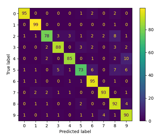
Confusion Matrix
On this method, we are able to see that the courses with the bottom efficiency are 5 and a couple of, that are mistaken principally for 8.
Your entire code itemizing is as follows:
from cv2 import ml
from sklearn.datasets import make_blobs
from sklearn import model_selection as ms
from sklearn.metrics import confusion_matrix, ConfusionMatrixDisplay
from numpy import float32
from matplotlib.pyplot import present
from digits_dataset import split_images, split_data
# Load the digits picture
img, sub_imgs = split_images(‘Photos/digits.png’, 20)
# Get hold of coaching and testing datasets from the digits picture
digits_train_imgs, digits_train_labels, digits_test_imgs, digits_test_labels = split_data(20, sub_imgs, 0.8)
# Create an empty logistic regression mannequin
lr_digits = ml.LogisticRegression_create()
# Verify the default coaching methodology
print(‘Coaching Methodology:’, lr_digits.getTrainMethod())
# Set the coaching methodology to Mini-Batch Gradient Descent and the scale of the mini-batch
lr_digits.setTrainMethod(ml.LogisticRegression_MINI_BATCH)
lr_digits.setMiniBatchSize(400)
# Set the variety of iterations
lr_digits.setIterations(10)
# Prepare the logistic regressor on the set of coaching information
lr_digits.practice(digits_train_imgs.astype(float32), ml.ROW_SAMPLE, digits_train_labels.astype(float32))
# Print the variety of discovered coefficients, and the variety of enter options
print(‘Variety of coefficients:’, len(lr_digits.get_learnt_thetas()[0]))
print(‘Variety of enter options:’, len(digits_train_imgs[0, :]))
# Predict the goal labels of the testing information
_, y_pred = lr_digits.predict(digits_test_imgs.astype(float32))
# Compute and print the achieved accuracy
accuracy = (sum(y_pred[:, 0] == digits_test_labels[:, 0]) / digits_test_labels.dimension) * 100
print(‘Accuracy:’, accuracy, ‘%’)
# Generate and plot confusion matrix
cm = confusion_matrix(digits_test_labels, y_pred)
disp = ConfusionMatrixDisplay(confusion_matrix=cm)
disp.plot()
present()
1
2
3
4
5
6
7
8
9
10
11
12
13
14
15
16
17
18
19
20
21
22
23
24
25
26
27
28
29
30
31
32
33
34
35
36
37
38
39
40
41
42
43
44
45
46
from cv2 import ml
from sklearn.datasets import make_blobs
from sklearn import model_selection as ms
from sklearn.metrics import confusion_matrix, ConfusionMatrixDisplay
from numpy import float32
from matplotlib.pyplot import present
from digits_dataset import split_images, cut up_information
# Load the digits picture
img, sub_imgs = split_images(‘Photos/digits.png’, 20)
# Get hold of coaching and testing datasets from the digits picture
digits_train_imgs, digits_train_labels, digits_test_imgs, digits_test_labels = split_data(20, sub_imgs, 0.8)
# Create an empty logistic regression mannequin
lr_digits = ml.LogisticRegression_create()
# Verify the default coaching methodology
print(‘Coaching Methodology:’, lr_digits.getTrainMethod())
# Set the coaching methodology to Mini-Batch Gradient Descent and the scale of the mini-batch
lr_digits.setTrainMethod(ml.LogisticRegression_MINI_BATCH)
lr_digits.setMiniBatchSize(400)
# Set the variety of iterations
lr_digits.setIterations(10)
# Prepare the logistic regressor on the set of coaching information
lr_digits.practice(digits_train_imgs.astype(float32), ml.ROW_SAMPLE, digits_train_labels.astype(float32))
# Print the variety of discovered coefficients, and the variety of enter options
print(‘Variety of coefficients:’, len(lr_digits.get_learnt_thetas()[0]))
print(‘Variety of enter options:’, len(digits_train_imgs[0, :]))
# Predict the goal labels of the testing information
_, y_pred = lr_digits.predict(digits_test_imgs.astype(float32))
# Compute and print the achieved accuracy
accuracy = (sum(y_pred[:, 0] == digits_test_labels[:, 0]) / digits_test_labels.dimension) * 100
print(‘Accuracy:’, accuracy, ‘%’)
# Generate and plot confusion matrix
cm = confusion_matrix(digits_test_labels, y_pred)
disp = ConfusionMatrixDisplay(confusion_matrix=cm)
disp.plot()
present()
On this tutorial, now we have utilized the logistic regression methodology, inherently designed for binary classification, to a multi-class classification downside. We have now used the pixel values as enter options representing every picture, acquiring an 88.8% classification accuracy with the chosen parameter values.
How about testing whether or not coaching the logistic regression algorithm on HOG descriptors extracted from the photographs would enhance this accuracy?
Additional Studying
This part offers extra sources on the subject if you wish to go deeper.
Books
Web sites
Abstract
On this tutorial, you discovered how the usual logistic regression algorithm, inherently designed for binary classification, will be modified to cater to multi-class classification issues by making use of it to a picture classification process.
Particularly, you discovered:
A number of of crucial traits of the logistic regression algorithm.
How the logistic regression algorithm will be modified for multi-class classification issues.
Tips on how to apply logistic regression to the issue of picture classification.
Do you could have any questions?
Ask your questions within the feedback beneath, and I’ll do my greatest to reply.


 May One Up the Pixel 7a and Galaxy A54 in Price | nextpit")


")

")


/cdn.vox-cdn.com/uploads/chorus_asset/file/25661290/Screenshot_2024_10_06_at_10.48.36_AM.png "Trailers of the week: Nosferatu, The Franchise, and Squid Game 2")


