

The Naive Bayes algorithm is an easy however highly effective approach for supervised machine studying. Its Gaussian variant is carried out within the OpenCV library.
On this tutorial, you’ll discover ways to apply OpenCV’s regular Bayes algorithm, first on a customized two-dimensional dataset and subsequently for segmenting a picture.
After finishing this tutorial, you’ll know:
A number of of a very powerful factors in making use of the Bayes theorem to machine studying.
The right way to use the traditional Bayes algorithm on a customized dataset in OpenCV.
The right way to use the traditional Bayes algorithm to section a picture in OpenCV.
Let’s get began.
Regular Bayes Classifier for Picture Segmentation Utilizing OpenCV Photograph by Fabian Irsara, some rights reserved.
Tutorial Overview
This tutorial is split into three components; they’re:
Reminder of the Bayes Theorem As Utilized to Machine Studying
Discovering Bayes Classification in OpenCV
Picture Segmentation Utilizing a Regular Bayes Classifier
Reminder of the Bayes Theorem As Utilized to Machine Studying
This tutorial by Jason Brownlee provides an in-depth clarification of Bayes Theorem for machine studying, so let’s first begin with brushing up on a number of the most necessary factors from his tutorial:
The Bayes Theorem is beneficial in machine studying as a result of it gives a statistical mannequin to formulate the connection between information and a speculation.
Expressed as $P(h | D) = P(D | h) * P(h) / P(D)$, the Bayes Theorem states that the likelihood of a given speculation being true (denoted by $P(h | D)$ and often known as the posterior likelihood of the speculation) will be calculated by way of:
The likelihood of observing the info given the speculation (denoted by $P(D | h)$ and often known as the chance).
The likelihood of the speculation being true, independently of the info (denoted by $P(h)$ and often known as the prior likelihood of the speculation).
The likelihood of observing the info independently of the speculation (denoted by $P(D)$ and often known as the proof).
The Bayes Theorem assumes that each variable (or function) making up the enter information, $D$, is dependent upon all the opposite variables (or options).
Inside the context of information classification, the Bayes Theorem could also be utilized to the issue of calculating the conditional likelihood of a category label given a knowledge pattern: $P(class | information) = P(information | class) * P(class) / P(information)$, the place the category label now substitutes the speculation. The proof, $P(information)$, is a continuing and will be dropped.
Within the formulation of the issue as outlined within the bullet level above, the estimation of the chance, $P(information | class)$, will be troublesome as a result of it requires that the variety of information samples is sufficiently giant to comprise all attainable combos of variables (or options) for every class. That is seldom the case, particularly with high-dimensional information with many variables.
The formulation above will be simplified into what is called Naive Bayes, the place every enter variable is handled individually: $P(class | X_1, X_2, dots, X_n) = P(X_1 | class) * P(X_2 | class) * dots * P(X_n | class) * P(class)$
The Naive Bayes estimation adjustments the formulation from a dependent conditional likelihood mannequin to an unbiased conditional likelihood mannequin, the place the enter variables (or options) are actually assumed to be unbiased. This assumption not often holds with real-world information, therefore the title naive.
Discovering Bayes Classification in OpenCV
Suppose the enter information we’re working with is steady. In that case, it might be modeled utilizing a steady likelihood distribution, corresponding to a Gaussian (or regular) distribution, the place the info belonging to every class is modeled by its imply and commonplace deviation.
The Bayes classifier carried out in OpenCV is a traditional Bayes classifier (additionally generally often known as Gaussian Naive Bayes), which assumes that the enter options from every class are usually distributed.
This easy classification mannequin assumes that function vectors from every class are usually distributed (although, not essentially independently distributed).
– OpenCV, Machine Studying Overview, 2023.
To find easy methods to use the traditional Bayes classifier in OpenCV, let’s begin by testing it on a easy two-dimensional dataset as we did in earlier tutorials.
For this goal, let’s generate a dataset consisting of 100 information factors (specified by n_samples), that are equally divided into 2 Gaussian clusters (recognized by facilities) having a typical deviation set to 1.5 (specified by cluster_std). Let’s additionally outline a price for random_state to have the ability to replicate the outcomes:
# Producing a dataset of 2D information factors and their floor reality labels
x, y_true = make_blobs(n_samples=100, facilities=2, cluster_std=1.5, random_state=15)
# Plotting the dataset
scatter(x[:, 0], x[:, 1], c=y_true)
present()
# Producing a dataset of 2D information factors and their floor reality labels
x, y_true = make_blobs(n_samples=100, facilities=2, cluster_std=1.5, random_state=15)
# Plotting the dataset
scatter(x[:, 0], x[:, 1], c=y_true)
present()
The code above ought to generate the next plot of information factors:
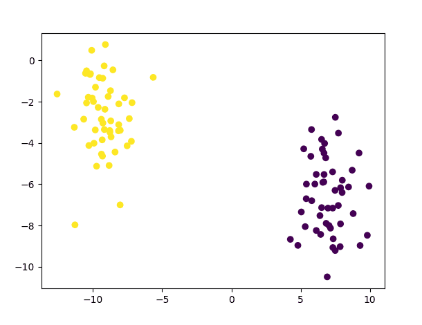
Scatter Plot of Dataset Consisting of two Gaussian Clusters
We will then break up this dataset, allocating 80% of the info to the coaching set and the remaining 20% to the take a look at set:
# Break up the info into coaching and testing units
x_train, x_test, y_train, y_test = ms.train_test_split(x, y_true, test_size=0.2, random_state=10)
# Break up the info into coaching and testing units
x_train, x_test, y_train, y_test = ms.train_test_split(x, y_true, test_size=0.2, random_state=10)
Following this, we are going to create the traditional Bayes classifier and proceed with coaching and testing it on the dataset values after having sort solid to 32-bit float:
# Create a brand new Regular Bayes Classifier
norm_bayes = ml.NormalBayesClassifier_create()
# Practice the classifier on the coaching information
norm_bayes.prepare(x_train.astype(float32), ml.ROW_SAMPLE, y_train)
# Generate a prediction from the educated classifier
ret, y_pred, y_probs = norm_bayes.predictProb(x_test.astype(float32))
By making use of the predictProb technique, we are going to acquire the expected class for every enter vector (with every vector being saved on every row of the array fed into the traditional Bayes classifier) and the output chances.
Within the code above, the expected courses are saved in y_pred, whereas y_probs is an array with as many columns as courses (two on this case) that holds the likelihood worth of every enter vector belonging to every class into consideration. It might make sense that the output likelihood values the classifier returns for every enter vector sum as much as one. Nevertheless, this may occasionally not essentially be the case as a result of the likelihood values the classifier returns aren’t normalized by the proof, $P(information)$, which we now have faraway from the denominator, as defined within the earlier part.
As a substitute, what’s being reported is a chance, which is principally the numerator of the conditional likelihood equation, p(C) p(M | C). The denominator, p(M), doesn’t must be computed.
– Machine Studying for OpenCV, 2017.
Nonetheless, whether or not the values are normalized or not, the category prediction for every enter vector could also be discovered by figuring out the category with the very best likelihood worth.
The code itemizing thus far is the next:
from sklearn.datasets import make_blobs
from sklearn import model_selection as ms
from numpy import float32
from matplotlib.pyplot import scatter, present
from cv2 import ml
# Generate a dataset of 2D information factors and their floor reality labels
x, y_true = make_blobs(n_samples=100, facilities=2, cluster_std=1.5, random_state=15)
# Plot the dataset
scatter(x[:, 0], x[:, 1], c=y_true)
present()
# Break up the info into coaching and testing units
x_train, x_test, y_train, y_test = ms.train_test_split(x, y_true, test_size=0.2, random_state=10)
# Create a brand new Regular Bayes Classifier
norm_bayes = ml.NormalBayesClassifier_create()
# Practice the classifier on the coaching information
norm_bayes.prepare(x_train.astype(float32), ml.ROW_SAMPLE, y_train)
# Generate a prediction from the educated classifier
ret, y_pred, y_probs = norm_bayes.predictProb(x_test.astype(float32))
# Plot the category predictions
scatter(x_test[:, 0], x_test[:, 1], c=y_pred)
present()
1
2
3
4
5
6
7
8
9
10
11
12
13
14
15
16
17
18
19
20
21
22
23
24
25
26
27
28
from sklearn.datasets import make_blobs
from sklearn import model_selection as ms
from numpy import float32
from matplotlib.pyplot import scatter, present
from cv2 import ml
# Generate a dataset of 2D information factors and their floor reality labels
x, y_true = make_blobs(n_samples=100, facilities=2, cluster_std=1.5, random_state=15)
# Plot the dataset
scatter(x[:, 0], x[:, 1], c=y_true)
present()
# Break up the info into coaching and testing units
x_train, x_test, y_train, y_test = ms.train_test_split(x, y_true, test_size=0.2, random_state=10)
# Create a brand new Regular Bayes Classifier
norm_bayes = ml.NormalBayesClassifier_create()
# Practice the classifier on the coaching information
norm_bayes.prepare(x_train.astype(float32), ml.ROW_SAMPLE, y_train)
# Generate a prediction from the educated classifier
ret, y_pred, y_probs = norm_bayes.predictProb(x_test.astype(float32))
# Plot the category predictions
scatter(x_test[:, 0], x_test[:, 1], c=y_pred)
present()
We might even see that the category predictions produced by the traditional Bayes classifier educated on this easy dataset are right:

Scatter Plot of Predictions Generated for the Take a look at Samples
Picture Segmentation Utilizing a Regular Bayes Classifier
Amongst their many functions, Bayes classifiers have been regularly used for pores and skin segmentation, which separates pores and skin pixels from non-skin pixels in a picture.
We will adapt the code above for segmenting pores and skin pixels in photos. For this goal, we are going to use the Pores and skin Segmentation dataset, consisting of fifty,859 pores and skin samples and 194,198 non-skin samples, to coach the traditional Bayes classifier. The dataset presents the pixel values in BGR order and their corresponding class label.
After loading the dataset, we will convert the BGR pixel values into HSV (denoting Hue, Saturation, and Worth) after which use the hue values to coach a traditional Bayes classifier. Hue is usually most well-liked over RGB in picture segmentation duties as a result of it represents the true coloration with out modification and is much less affected by lighting variations than RGB. Within the HSV coloration mannequin, the hue values are organized radially and span between 0 and 360 levels:
from cv2 import ml,
from numpy import loadtxt, float32
from matplotlib.colours import rgb_to_hsv
# Load information from textual content file
information = loadtxt(“Information/Skin_NonSkin.txt”, dtype=int)
# Choose the BGR values from the loaded information
BGR = information[:, :3]
# Convert to RGB by swapping the array columns
RGB = BGR.copy()
RGB[:, [2, 0]] = RGB[:, [0, 2]]
# Convert RGB values to HSV
HSV = rgb_to_hsv(RGB.reshape(RGB.form[0], -1, 3) / 255)
HSV = HSV.reshape(RGB.form[0], 3)
# Choose solely the hue values
hue = HSV[:, 0] * 360
# Choose the labels from the loaded information
labels = information[:, -1]
# Create a brand new Regular Bayes Classifier
norm_bayes = ml.NormalBayesClassifier_create()
# Practice the classifier on the hue values
norm_bayes.prepare(hue.astype(float32), ml.ROW_SAMPLE, labels)
1
2
3
4
5
6
7
8
9
10
11
12
13
14
15
16
17
18
19
20
21
22
23
24
25
26
27
28
29
from cv2 import ml,
from numpy import loadtxt, float32
from matplotlib.colours import rgb_to_hsv
# Load information from textual content file
information = loadtxt(“Information/Skin_NonSkin.txt”, dtype=int)
# Choose the BGR values from the loaded information
BGR = information[:, :3]
# Convert to RGB by swapping the array columns
RGB = BGR.copy()
RGB[:, [2, 0]] = RGB[:, [0, 2]]
# Convert RGB values to HSV
HSV = rgb_to_hsv(RGB.reshape(RGB.form[0], –1, 3) / 255)
HSV = HSV.reshape(RGB.form[0], 3)
# Choose solely the hue values
hue = HSV[:, 0] * 360
# Choose the labels from the loaded information
labels = information[:, –1]
# Create a brand new Regular Bayes Classifier
norm_bayes = ml.NormalBayesClassifier_create()
# Practice the classifier on the hue values
norm_bayes.prepare(hue.astype(float32), ml.ROW_SAMPLE, labels)
Observe 1: The OpenCV library gives the cvtColor technique to transform between coloration areas, as seen on this tutorial, however the cvtColor technique expects the supply picture in its unique form as an enter. The rgb_to_hsv technique in Matplotlib, however, accepts a NumPy array within the type of (…, 3) as enter, the place the array values are anticipated to be normalized throughout the vary of 0 to 1. We’re utilizing the latter right here since our coaching information consists of particular person pixels, which aren’t structured within the common type of a three-channel picture.
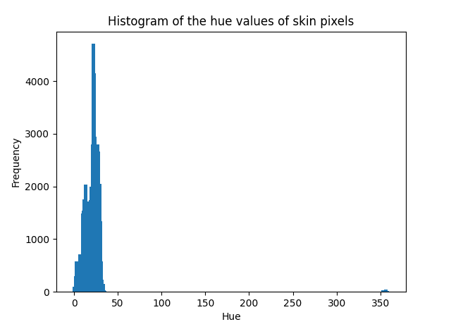
Observe 2: The conventional Bayes classifier assumes that the info to be modeled follows a Gaussian distribution. Whereas this isn’t a strict requirement, the classifier’s efficiency could degrade if the info is distributed in any other case. We could examine the distribution of the info we’re working with by plotting its histogram. If we take the hue values of the pores and skin pixels for example, we discover {that a} Gaussian curve can describe their distribution:
from numpy import histogram
from matplotlib.pyplot import bar, title, xlabel, ylabel, present
# Select the skin-labelled hue values
pores and skin = x[labels == 1]
# Compute their histogram
hist, bin_edges = histogram(pores and skin, vary=[0, 360], bins=360)
# Show the computed histogram
bar(bin_edges[:-1], hist, width=4)
xlabel(‘Hue’)
ylabel(‘Frequency’)
title(‘Histogram of the hue values of pores and skin pixels’)
present()
from numpy import histogram
from matplotlib.pyplot import bar, title, xlabel, ylabel, present
# Select the skin-labelled hue values
pores and skin = x[labels == 1]
# Compute their histogram
hist, bin_edges = histogram(pores and skin, vary=[0, 360], bins=360)
# Show the computed histogram
bar(bin_edges[:–1], hist, width=4)
xlabel(‘Hue’)
ylabel(‘Frequency’)
title(‘Histogram of the hue values of pores and skin pixels’)
present()
Checking the Distribution of the Information
As soon as the traditional Bayes classifier has been educated, we could check it out on a picture (let’s think about this instance picture for testing):
from cv2 import imread
from matplotlib.pyplot import present, imshow
# Load a take a look at picture
face_img = imread(“Photographs/face.jpg”)
# Reshape the picture right into a three-column array
face_BGR = face_img.reshape(-1, 3)
# Convert to RGB by swapping the array columns
face_RGB = face_BGR.copy()
face_RGB[:, [2, 0]] = face_RGB[:, [0, 2]]
# Convert from RGB to HSV
face_HSV = rgb_to_hsv(face_RGB.reshape(face_RGB.form[0], -1, 3) / 255)
face_HSV = face_HSV.reshape(face_RGB.form[0], 3)
# Choose solely the hue values
face_hue = face_HSV[:, 0] * 360
# Show the hue picture
imshow(face_hue.reshape(face_img.form[0], face_img.form[1]))
present()
# Generate a prediction from the educated classifier
ret, labels_pred, output_probs = norm_bayes.predictProb(face_hue.astype(float32))
# Reshape array into the enter picture measurement and select the skin-labelled pixels
skin_mask = labels_pred.reshape(face_img.form[0], face_img.form[1], 1) == 1
# Show the segmented picture
imshow(skin_mask, cmap=’grey’)
present()
1
2
3
4
5
6
7
8
9
10
11
12
13
14
15
16
17
18
19
20
21
22
23
24
25
26
27
28
29
30
31
32
33
from cv2 import imread
from matplotlib.pyplot import present, imshow
# Load a take a look at picture
face_img = imread(“Photographs/face.jpg”)
# Reshape the picture right into a three-column array
face_BGR = face_img.reshape(–1, 3)
# Convert to RGB by swapping the array columns
face_RGB = face_BGR.copy()
face_RGB[:, [2, 0]] = face_RGB[:, [0, 2]]
# Convert from RGB to HSV
face_HSV = rgb_to_hsv(face_RGB.reshape(face_RGB.form[0], –1, 3) / 255)
face_HSV = face_HSV.reshape(face_RGB.form[0], 3)
# Choose solely the hue values
face_hue = face_HSV[:, 0] * 360
# Show the hue picture
imshow(face_hue.reshape(face_img.form[0], face_img.form[1]))
present()
# Generate a prediction from the educated classifier
ret, labels_pred, output_probs = norm_bayes.predictProb(face_hue.astype(float32))
# Reshape array into the enter picture measurement and select the skin-labelled pixels
skin_mask = labels_pred.reshape(face_img.form[0], face_img.form[1], 1) == 1
# Show the segmented picture
imshow(skin_mask, cmap=‘grey’)
present()
The ensuing segmented masks shows the pixels labeled as belonging to the pores and skin (with a category label equal to 1).
By qualitatively analyzing the consequence, we might even see that a lot of the pores and skin pixels have been accurately labeled as such. We can also see that some hair strands (therefore, non-skin pixels) have been incorrectly labeled as belonging to pores and skin. If we had to take a look at their hue values, we’d discover that these are similar to these belonging to pores and skin areas, therefore the mislabelling. Moreover, we can also discover the effectiveness of utilizing the hue values, which stay comparatively fixed in areas of the face that in any other case seem illuminated or in shadow within the unique RGB picture:
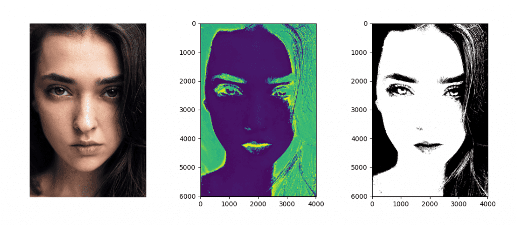
Authentic Picture (Left); Hue Values (Center); Segmented Pores and skin Pixels (Proper)
Are you able to consider extra exams to check out with a traditional Bayes classifier?
Additional Studying
This part gives extra assets on the subject if you wish to go deeper.
Books
Abstract
On this tutorial, you discovered easy methods to apply OpenCV’s regular Bayes algorithm, first on a customized two-dimensional dataset and subsequently for segmenting a picture.
Particularly, you discovered:
A number of of a very powerful factors in making use of the Bayes theorem to machine studying.
The right way to use the traditional Bayes algorithm on a customized dataset in OpenCV.
The right way to use the traditional Bayes algorithm to section a picture in OpenCV.
Do you will have any questions?
Ask your questions within the feedback beneath, and I’ll do my finest to reply.


")

")


