

Utilizing a Haar cascade classifier in OpenCV is easy. You simply want to offer the educated mannequin in an XML file to create the classifier. Coaching one from scratch, nonetheless, just isn’t so simple. On this tutorial, you will notice how the coaching ought to be like. Specifically, you’ll be taught:
What are the instruments to coach a Haar cascade in OpenCV
Find out how to put together information for coaching
Find out how to run the coaching
Kick-start your mission with my e book Machine Studying in OpenCV. It supplies self-study tutorials with working code.
Let’s get began.
Coaching a Haar Cascade Object Detector in OpenCVPhoto by Adrià Crehuet Cano. Some rights reserved.
Overview
This put up is split into 5 components; they’re:
The Downside of Coaching Cascade Classifier in OpenCV
Setup of Atmosphere
Overview of the Coaching of Cascade Classifier
Put together Coaching DAta
Coaching Haar Cascade Classifier
The Downside of Coaching Cascade Classifier in OpenCV
OpenCV has been round for a few years and has many variations. OpenCV 5 is in improvement on the time of writing and the really helpful model is OpenCV 4, or model 4.8.0, to be exact.
There was a number of clean-up between OpenCV 3 and OpenCV 4. Most notably a considerable amount of code has been rewritten. The change is substantial and fairly a lot of features are modified. This included the instrument to coach the Haar cascade classifier.
A cascade classifier just isn’t a easy mannequin like SVM that you could practice simply. It’s an ensemble mannequin that makes use of AdaBoost. Due to this fact, the coaching entails a number of steps. OpenCV 3 has a command line instrument to assist do such coaching, however the instrument has been damaged in OpenCV 4. The repair just isn’t accessible but.
Due to this fact, it is just attainable to coach a Haar cascade classifier utilizing OpenCV 3. Happily, you may discard it after the coaching and revert to OpenCV 4 when you save the mannequin in an XML file. That is what you’re going to do on this put up.
You can not have OpenCV 3 and OpenCV 4 co-exist in Python. Due to this fact, it’s endorsed to create a separate surroundings for coaching. In Python, you should use the venv module to create a digital surroundings, which is solely to create a separate set of put in modules. Options can be utilizing Anaconda or Pyenv, that are totally different architectures beneath the identical philosophy. Amongst all the above, you must see the Anaconda surroundings as the best for this job.
Setup of Atmosphere
It’s simpler should you’re utilizing Anaconda, you should use the next command to create and use a brand new surroundings and identify it as “cvtrain”:
conda create -n cvtrain python ‘opencv>=3,<4’
conda activate cvtrain
conda create –n cvtrain python ‘opencv>=3,<4’
conda activate cvtrain
You already know you’re prepared should you discover the command opencv_traincascade is obtainable:
$ opencv_traincascade
Utilization: opencv_traincascade
-data <cascade_dir_name>
-vec <vec_file_name>
-bg <background_file_name>
[-numPos <number_of_positive_samples = 2000>]
[-numNeg <number_of_negative_samples = 1000>]
[-numStages <number_of_stages = 20>]
[-precalcValBufSize <precalculated_vals_buffer_size_in_Mb = 1024>]
[-precalcIdxBufSize <precalculated_idxs_buffer_size_in_Mb = 1024>]
[-baseFormatSave]
[-numThreads <max_number_of_threads = 16>]
[-acceptanceRatioBreakValue <value> = -1>]
–cascadeParams–
[-stageType <BOOST(default)>]
[-featureType <{HAAR(default), LBP, HOG}>]
[-w <sampleWidth = 24>]
[-h <sampleHeight = 24>]
–boostParams–
[-bt <{DAB, RAB, LB, GAB(default)}>]
[-minHitRate <min_hit_rate> = 0.995>]
[-maxFalseAlarmRate <max_false_alarm_rate = 0.5>]
[-weightTrimRate <weight_trim_rate = 0.95>]
[-maxDepth <max_depth_of_weak_tree = 1>]
[-maxWeakCount <max_weak_tree_count = 100>]
–haarFeatureParams–
[-mode <BASIC(default) | CORE | ALL
–lbpFeatureParams–
–HOGFeatureParams–
1
2
3
4
5
6
7
8
9
10
11
12
13
14
15
16
17
18
19
20
21
22
23
24
25
26
27
28
29
$ opencv_traincascade
Usage: opencv_traincascade
–data <cascade_dir_name>
–vec <vec_file_name>
–bg <background_file_name>
[–numPos <number_of_positive_samples = 2000>]
[–numNeg <number_of_negative_samples = 1000>]
[–numStages <number_of_stages = 20>]
[–precalcValBufSize <precalculated_vals_buffer_size_in_Mb = 1024>]
[–precalcIdxBufSize <precalculated_idxs_buffer_size_in_Mb = 1024>]
[–baseFormatSave]
[–numThreads <max_number_of_threads = 16>]
[–acceptanceRatioBreakValue <value> = –1>]
—cascadeParams—
[–stageType <BOOST(default)>]
[–featureType <{HAAR(default), LBP, HOG}>]
[–w <sampleWidth = 24>]
[–h <sampleHeight = 24>]
—boostParams—
[–bt <{DAB, RAB, LB, GAB(default)}>]
[–minHitRate <min_hit_rate> = 0.995>]
[–maxFalseAlarmRate <max_false_alarm_rate = 0.5>]
[–weightTrimRate <weight_trim_rate = 0.95>]
[–maxDepth <max_depth_of_weak_tree = 1>]
[–maxWeakCount <max_weak_tree_count = 100>]
—haarFeatureParams—
[–mode <BASIC(default) | CORE | ALL
—lbpFeatureParams—
—HOGFeatureParams—
If you’re using pyenv or venv, you need more steps. First, create an environment and install OpenCV (you should notice the different name of the package than Anaconda ecosystem):
# create an environment and install opencv 3
pyenv virtualenv 3.11 cvtrain
pyenv activate cvtrain
pip install ‘opencv-python>=3,<4’
# create an environment and install opencv 3
pyenv virtualenv 3.11 cvtrain
pyenv activate cvtrain
pip install ‘opencv-python>=3,<4’
This allows you to run Python programs using OpenCV but you do not have the command line tools for training. To get the tools, you need to compile them from source code by following these steps:
Download OpenCV source code and switch to 3.4 branch
# download OpenCV source code and switch to 3.4 branch
git clone https://github.com/opencv/opencv
cd opencv
git checkout 3.4
cd ..
# download OpenCV source code and switch to 3.4 branch
git clone https://github.com/opencv/opencv
cd opencv
git checkout 3.4
cd ..
Create the build directory separate from the repository directory:
Prepare the build directory with cmake tool, and referring to the OpenCV repository:
Run make to compile (you may need to have the developer libraries installed in your system first)
The tools you need will be in the bin/ directory, as shown by the last command above
The command line tools needed are opencv_traincascade and opencv_createsamples. The rest of this post assumes you have these tools available.
Overview of the Training of Cascade Classifier
You are going to train a cascade classifier using OpenCV tools. The classifier is an ensemble model using AdaBoost. Simply, multiple smaller models are created where each of them is weak in classification. Combined, it becomes a strong classifier with a good rates of precision and recall.
Each of the weak classifiers is a binary classifier. To train them, you need some positive samples and negative samples. The negative samples are easy: You provide some random pictures to OpenCV and let OpenCV select a rectangular region (better if there are no target objects in these pictures). The positive samples, however, are provided as an image and the bounding box in which the object lies perfectly in the box.
Once these datasets are provided, OpenCV will extract the Haar features from both and use them to train many classifiers. Haar features are from partitioning the positive or negative samples into rectangular regions. How the partitioning is done involves some randomness. Therefore, it takes time for OpenCV to find the best way to derive the Haar features for this classification task.
In OpenCV, you just need to provide the training data in image files in a format that OpenCV can read (such as JPEG or PNG). For negative samples, all it needs is a plain text file of their filenames. For positive samples, an “info file” is required, which is a plaintext file with the details of the filename, how many objects are in the picture, and the corresponding bounding boxes.
The positive data samples for training should be in a binary format. OpenCV provides a tool opencv_createsamples to generate the binary format from the “info file”. Then these positive samples, together with the negative samples, are provided to another tool opencv_traincascade to run the training and produce the model output in the format of an XML file. This is the XML file you can load into a OpenCV Haar cascade classifier.
Prepare Training Data
Let’s consider creating a cat face detector. To train such a detector, you need the dataset first. One possibility is the Oxford-IIIT Pet Dataset, at this location:
This is an 800MB dataset, a small one by the standards of computer vision datasets. The images are annotated in the Pascal VOC format. In short, each image has a corresponding XML file that looks like the following:
<?xml version=”1.0″?>
<annotation>
<folder>OXIIIT</folder>
<filename>Abyssinian_100.jpg</filename>
<source>
<database>OXFORD-IIIT Pet Dataset</database>
<annotation>OXIIIT</annotation>
<image>flickr</image>
</source>
<size>
<width>394</width>
<height>500</height>
<depth>3</depth>
</size>
<segmented>0</segmented>
<object>
<name>cat</name>
<pose>Frontal</pose>
<truncated>0</truncated>
<occluded>0</occluded>
<bndbox>
<xmin>151</xmin>
<ymin>71</ymin>
<xmax>335</xmax>
<ymax>267</ymax>
</bndbox>
<difficult>0</difficult>
</object>
</annotation>
1
2
3
4
5
6
7
8
9
10
11
12
13
14
15
16
17
18
19
20
21
22
23
24
25
26
27
28
29
<?xml version=“1.0”?>
<annotation>
<folder>OXIIIT</folder>
<filename>Abyssinian_100.jpg</filename>
<source>
<database>OXFORD-IIIT Pet Dataset</database>
<annotation>OXIIIT</annotation>
<image>flickr</image>
</source>
<size>
<width>394</width>
<height>500</height>
<depth>3</depth>
</size>
<segmented>0</segmented>
<object>
<name>cat</name>
<pose>Frontal</pose>
<truncated>0</truncated>
<occluded>0</occluded>
<bndbox>
<xmin>151</xmin>
<ymin>71</ymin>
<xmax>335</xmax>
<ymax>267</ymax>
</bndbox>
<difficult>0</difficult>
</object>
</annotation>
The XML file tells you which image file it is referring to (Abyssinian_100.jpg in the example above), and what object it contains, with the bounding box between the tags <bndbox></bndbox>.
To extract the bounding boxes from the XML file, you can use the following function:
import xml.etree.ElementTree as ET
def read_voc_xml(xmlfile: str) -> dict:
root = ET.parse(xmlfile).getroot()
boxes = {“filename”: root.find(“filename”).text,
“objects”: []}
for field in root.iter(‘object’):
bb = field.discover(‘bndbox’)
obj = {
“identify”: field.discover(‘identify’).textual content,
“xmin”: int(bb.discover(“xmin”).textual content),
“ymin”: int(bb.discover(“ymin”).textual content),
“xmax”: int(bb.discover(“xmax”).textual content),
“ymax”: int(bb.discover(“ymax”).textual content),
}
packing containers[“objects”].append(obj)
return packing containers
1
2
3
4
5
6
7
8
9
10
11
12
13
14
15
16
17
18
import xml.etree.ElementTree as ET
def read_voc_xml(xmlfile: str) -> dict:
root = ET.parse(xmlfile).getroot()
packing containers = {“filename”: root.discover(“filename”).textual content,
“objects”: []}
for field in root.iter(‘object’):
bb = field.discover(‘bndbox’)
obj = {
“identify”: field.discover(‘identify’).textual content,
“xmin”: int(bb.discover(“xmin”).textual content),
“ymin”: int(bb.discover(“ymin”).textual content),
“xmax”: int(bb.discover(“xmax”).textual content),
“ymax”: int(bb.discover(“ymax”).textual content),
}
packing containers[“objects”].append(obj)
return packing containers
An instance of the dictionary returned by the above operate is as follows:
{‘filename’: ‘yorkshire_terrier_160.jpg’,
‘objects’: [{‘name’: ‘dog’, ‘xmax’: 290, ‘xmin’: 97, ‘ymax’: 245, ‘ymin’: 18}]}
{‘filename’: ‘yorkshire_terrier_160.jpg’,
‘objects’: [{‘name’: ‘dog’, ‘xmax’: 290, ‘xmin’: 97, ‘ymax’: 245, ‘ymin’: 18}]}
With these, it’s straightforward to create the dataset for the coaching: Within the Oxford-IIT Pet dataset, the pictures are both cats or canine. You’ll be able to let all canine pictures as detrimental samples. Then all of the cat pictures can be optimistic samples with acceptable bounding field set.
The “information file” that OpenCV expects for optimistic samples is a plaintext file with every line within the following format:
filename N x0 y0 w0 h0 x1 y1 w1 h1 …
filename N x0 y0 w0 h0 x1 y1 w1 h1 …
The quantity following the filename is the depend of bounding packing containers on that picture. Every bounding field is a optimistic pattern. What follows it are the bounding packing containers. Every field is specified by the pixel coordinate at its high left nook and the width and top of the field. For the perfect results of the Haar cascade classifier, the bounding field ought to be in the identical side ratio because the mannequin expects.
Assume the Pet dataset you downloaded is positioned within the listing dataset/, which you must see the information are organized like the next:
dataset
|– annotations
| |– README
| |– listing.txt
| |– check.txt
| |– trainval.txt
| |– trimaps
| | |– Abyssinian_1.png
| | |– Abyssinian_10.png
| | …
| | |– yorkshire_terrier_98.png
| | `– yorkshire_terrier_99.png
| `– xmls
| |– Abyssinian_1.xml
| |– Abyssinian_10.xml
| …
| |– yorkshire_terrier_189.xml
| `– yorkshire_terrier_190.xml
`– photographs
|– Abyssinian_1.jpg
|– Abyssinian_10.jpg
…
|– yorkshire_terrier_98.jpg
`– yorkshire_terrier_99.jpg
1
2
3
4
5
6
7
8
9
10
11
12
13
14
15
16
17
18
19
20
21
22
23
24
dataset
|— annotations
| |— README
| |— listing.txt
| |— check.txt
| |— trainval.txt
| |— trimaps
| | |— Abyssinian_1.png
| | |— Abyssinian_10.png
| | ...
| | |— yorkshire_terrier_98.png
| | `— yorkshire_terrier_99.png
| `— xmls
| |— Abyssinian_1.xml
| |— Abyssinian_10.xml
| ...
| |— yorkshire_terrier_189.xml
| `— yorkshire_terrier_190.xml
`— photographs
|— Abyssinian_1.jpg
|— Abyssinian_10.jpg
...
|— yorkshire_terrier_98.jpg
`— yorkshire_terrier_99.jpg
With this, it’s straightforward to create the “information file” for optimistic samples and the listing of detrimental pattern information, utilizing the next program:
import pathlib
import xml.etree.ElementTree as ET
import numpy as np
def read_voc_xml(xmlfile: str) -> dict:
“””learn the Pascal VOC XML and return (filename, object identify, bounding field)
the place bounding field is a vector of (xmin, ymin, xmax, ymax). The pixel
coordinates are 1-based.
“””
root = ET.parse(xmlfile).getroot()
packing containers = {“filename”: root.discover(“filename”).textual content,
“objects”: []
}
for field in root.iter(‘object’):
bb = field.discover(‘bndbox’)
obj = {
“identify”: field.discover(‘identify’).textual content,
“xmin”: int(bb.discover(“xmin”).textual content),
“ymin”: int(bb.discover(“ymin”).textual content),
“xmax”: int(bb.discover(“xmax”).textual content),
“ymax”: int(bb.discover(“ymax”).textual content),
}
packing containers[“objects”].append(obj)
return packing containers
# Learn Pascal VOC and write information
base_path = pathlib.Path(“dataset”)
img_src = base_path / “photographs”
ann_src = base_path / “annotations” / “xmls”
detrimental = []
optimistic = []
for xmlfile in ann_src.glob(“*.xml”):
# load xml
ann = read_voc_xml(str(xmlfile))
if ann[‘objects’][0][‘name’] == ‘canine’:
# detrimental pattern (canine)
detrimental.append(str(img_src / ann[‘filename’]))
else:
# optimistic pattern (cats)
bbox = []
for obj in ann[‘objects’]:
x = obj[‘xmin’]
y = obj[‘ymin’]
w = obj[‘xmax’] – obj[‘xmin’]
h = obj[‘ymax’] – obj[‘ymin’]
bbox.append(f”{x} {y} {w} {h}”)
line = f”{str(img_src/ann[‘filename’])} {len(bbox)} {‘ ‘.be a part of(bbox)}”
optimistic.append(line)
# write the output to `detrimental.dat` and `postiive.dat`
with open(“detrimental.dat”, “w”) as fp:
fp.write(“n”.be a part of(detrimental))
with open(“optimistic.dat”, “w”) as fp:
fp.write(“n”.be a part of(optimistic))
1
2
3
4
5
6
7
8
9
10
11
12
13
14
15
16
17
18
19
20
21
22
23
24
25
26
27
28
29
30
31
32
33
34
35
36
37
38
39
40
41
42
43
44
45
46
47
48
49
50
51
52
53
54
55
56
57
58
import pathlib
import xml.etree.ElementTree as ET
import numpy as np
def read_voc_xml(xmlfile: str) -> dict:
“”“learn the Pascal VOC XML and return (filename, object identify, bounding field)
the place bounding field is a vector of (xmin, ymin, xmax, ymax). The pixel
coordinates are 1-based.
““”
root = ET.parse(xmlfile).getroot()
packing containers = {“filename”: root.discover(“filename”).textual content,
“objects”: []
}
for field in root.iter(‘object’):
bb = field.discover(‘bndbox’)
obj = {
“identify”: field.discover(‘identify’).textual content,
“xmin”: int(bb.discover(“xmin”).textual content),
“ymin”: int(bb.discover(“ymin”).textual content),
“xmax”: int(bb.discover(“xmax”).textual content),
“ymax”: int(bb.discover(“ymax”).textual content),
}
packing containers[“objects”].append(obj)
return packing containers
# Learn Pascal VOC and write information
base_path = pathlib.Path(“dataset”)
img_src = base_path / “photographs”
ann_src = base_path / “annotations” / “xmls”
detrimental = []
optimistic = []
for xmlfile in ann_src.glob(“*.xml”):
# load xml
ann = read_voc_xml(str(xmlfile))
if ann[‘objects’][0][‘name’] == ‘canine’:
# detrimental pattern (canine)
detrimental.append(str(img_src / ann[‘filename’]))
else:
# optimistic pattern (cats)
bbox = []
for obj in ann[‘objects’]:
x = obj[‘xmin’]
y = obj[‘ymin’]
w = obj[‘xmax’] – obj[‘xmin’]
h = obj[‘ymax’] – obj[‘ymin’]
bbox.append(f“{x} {y} {w} {h}”)
line = f“{str(img_src/ann[‘filename’])} {len(bbox)} {‘ ‘.be a part of(bbox)}”
optimistic.append(line)
# write the output to `detrimental.dat` and `postiive.dat`
with open(“detrimental.dat”, “w”) as fp:
fp.write(“n”.be a part of(detrimental))
with open(“optimistic.dat”, “w”) as fp:
fp.write(“n”.be a part of(optimistic))
This program scans all of the XML information from the dataset, then extracts the bounding packing containers from every if it’s a cat picture. The listing detrimental will maintain the paths to canine pictures. The listing optimistic will maintain the paths to cat pictures in addition to the bounding packing containers within the format described above, every line as one string. After the loop, these two lists are written to the disk as information detrimental.dat and optimistic.dat.
The content material of detrimental.dat is trivial. The content material of postiive.dat is like the next:
dataset/photographs/Siamese_102.jpg 1 154 92 194 176
dataset/photographs/Bengal_152.jpg 1 84 8 187 201
dataset/photographs/Abyssinian_195.jpg 1 8 6 109 115
dataset/photographs/Russian_Blue_135.jpg 1 228 90 103 117
dataset/photographs/Persian_122.jpg 1 60 16 230 228
dataset/photographs/Siamese_102.jpg 1 154 92 194 176
dataset/photographs/Bengal_152.jpg 1 84 8 187 201
dataset/photographs/Abyssinian_195.jpg 1 8 6 109 115
dataset/photographs/Russian_Blue_135.jpg 1 228 90 103 117
dataset/photographs/Persian_122.jpg 1 60 16 230 228
The step earlier than you run the coaching is to transform optimistic.dat right into a binary format. That is accomplished utilizing the next command line:
opencv_createsamples -info optimistic.dat -vec optimistic.vec -w 30 -h 30
opencv_createsamples –information optimistic.dat –vec optimistic.vec –w 30 –h 30
This command ought to be run in the identical listing as optimistic.dat such that the dataset photographs might be discovered. The output of this command can be optimistic.vec. It is usually generally known as the “vec file”. In doing so, that you must specify the width and top of the window utilizing -w and -h arguments. That is to resize the picture cropped by the bounding field into this pixel dimension earlier than writing to the vec file. This also needs to match the window dimension specified if you run the coaching.
Coaching Haar Cascade Classifier
Coaching a classifier takes time. It’s accomplished in a number of phases. Intermediate information are to be written in every stage, and as soon as all of the phases are accomplished, you’ll have the educated mannequin saved in an XML file. OpenCV expects all these generated information to be saved in a listing.
Run the coaching course of is certainly simple. Let’s take into account creating a brand new listing cat_detect to retailer the generated information. As soon as the listing is created, you may run the coaching utilizing the command line instrument opencv_traincascade:
# have to create the info dir first
mkdir cat_detect
# then run the coaching
opencv_traincascade -data cat_detect -vec optimistic.vec -bg detrimental.dat -numPos 900 -numNeg 2000 -numStages 10 -w 30 -h 30
# have to create the info dir first
mkdir cat_detect
# then run the coaching
opencv_traincascade –information cat_detect –vec optimistic.vec –bg detrimental.dat –numPos 900 –numNeg 2000 –numStages 10 –w 30 –h 30
Be aware using optimistic.vec as optimistic samples and detrimental.dat as detrimental samples. Additionally observe that, the -w and -h parameters are similar as what you used beforehand within the opencv_createsamples command. Different command line arguments are defined as follows:
-data <dirname>: The place the educated classifier is saved. This listing ought to exist already
-vec <filename>: The vec file of optimistic samples
-bg <filename>: The listing of detrimental samples, also referred to as “background” photographs
-numPos <N>: variety of optimistic samples utilized in coaching for each stage
-numNeg <N>: variety of detrimental samples utilized in coaching for each stage
-numStages <N>: variety of cascade phases to be educated
-w <width> and -h <top>: The pixel dimension for an object. This should be the identical as used throughout coaching samples creation with opencv_createsamples instrument
-minHitRate <fee>: The minimal desired true optimistic fee for every stage. Coaching a stage wouldn’t terminate till that is met.
-maxFalseAlarmRate <fee>: The utmost desired false optimistic fee for every stage. Coaching a stage wouldn’t terminate till that is met.
-maxDepth <N>: most depth of a weak tree
-maxWeakCount <N>: most variety of weak bushes for each stage
Not all of those arguments are required. However you must strive totally different combos to see should you can practice a greater detector.
Throughout coaching, you will notice the next display:
$ opencv_traincascade -data cat_detect -vec optimistic.vec -bg detrimental.dat -numPos 900 -numNeg 2000 -numStages 10 -w 30 -h 30
PARAMETERS:
cascadeDirName: cat_detect
vecFileName: optimistic.vec
bgFileName: detrimental.dat
numPos: 900
numNeg: 2000
numStages: 10
precalcValBufSize[Mb] : 1024
precalcIdxBufSize[Mb] : 1024
acceptanceRatioBreakValue : -1
stageType: BOOST
featureType: HAAR
sampleWidth: 30
sampleHeight: 30
boostType: GAB
minHitRate: 0.995
maxFalseAlarmRate: 0.5
weightTrimRate: 0.95
maxDepth: 1
maxWeakCount: 100
mode: BASIC
Variety of distinctive options given windowSize [30,30] : 394725
===== TRAINING 0-stage =====
<BEGIN
POS depend : consumed 900 : 900
NEG depend : acceptanceRatio 2000 : 1
Precalculation time: 3
+—-+———+———+
| N | HR | FA |
+—-+———+———+
| 1| 1| 1|
+—-+———+———+
| 2| 1| 1|
+—-+———+———+
| 3| 1| 1|
+—-+———+———+
| 4| 1| 0.8925|
+—-+———+———+
| 5| 0.998889| 0.7785|
…
| 19| 0.995556| 0.503|
+—-+———+———+
| 20| 0.995556| 0.492|
+—-+———+———+
END>
…
Coaching till now has taken 0 days 2 hours 55 minutes 44 seconds.
===== TRAINING 9-stage =====
<BEGIN
POS depend : consumed 900 : 948
NEG depend : acceptanceRatio 2000 : 0.00723552
Precalculation time: 4
+—-+———+———+
| N | HR | FA |
+—-+———+———+
| 1| 1| 1|
+—-+———+———+
| 2| 1| 1|
+—-+———+———+
| 3| 1| 1|
+—-+———+———+
| 4| 1| 1|
+—-+———+———+
| 5| 0.997778| 0.9895|
…
| 50| 0.995556| 0.5795|
+—-+———+———+
| 51| 0.995556| 0.4895|
+—-+———+———+
END>
Coaching till now has taken 0 days 3 hours 25 minutes 12 seconds.
1
2
3
4
5
6
7
8
9
10
11
12
13
14
15
16
17
18
19
20
21
22
23
24
25
26
27
28
29
30
31
32
33
34
35
36
37
38
39
40
41
42
43
44
45
46
47
48
49
50
51
52
53
54
55
56
57
58
59
60
61
62
63
64
65
66
67
68
69
70
71
72
73
74
$ opencv_traincascade -data cat_detect -vec optimistic.vec -bg detrimental.dat -numPos 900 -numNeg 2000 -numStages 10 -w 30 -h 30
PARAMETERS:
cascadeDirName: cat_detect
vecFileName: optimistic.vec
bgFileName: detrimental.dat
numPos: 900
numNeg: 2000
numStages: 10
precalcValBufSize[Mb] : 1024
precalcIdxBufSize[Mb] : 1024
acceptanceRatioBreakValue : -1
stageType: BOOST
featureType: HAAR
sampleWidth: 30
sampleHeight: 30
boostType: GAB
minHitRate: 0.995
maxFalseAlarmRate: 0.5
weightTrimRate: 0.95
maxDepth: 1
maxWeakCount: 100
mode: BASIC
Variety of distinctive options given windowSize [30,30] : 394725
===== TRAINING 0-stage =====
<BEGIN
POS depend : consumed 900 : 900
NEG depend : acceptanceRatio 2000 : 1
Precalculation time: 3
+—-+———+———+
| N | HR | FA |
+—-+———+———+
| 1| 1| 1|
+—-+———+———+
| 2| 1| 1|
+—-+———+———+
| 3| 1| 1|
+—-+———+———+
| 4| 1| 0.8925|
+—-+———+———+
| 5| 0.998889| 0.7785|
…
| 19| 0.995556| 0.503|
+—-+———+———+
| 20| 0.995556| 0.492|
+—-+———+———+
END>
…
Coaching till now has taken 0 days 2 hours 55 minutes 44 seconds.
===== TRAINING 9-stage =====
<BEGIN
POS depend : consumed 900 : 948
NEG depend : acceptanceRatio 2000 : 0.00723552
Precalculation time: 4
+—-+———+———+
| N | HR | FA |
+—-+———+———+
| 1| 1| 1|
+—-+———+———+
| 2| 1| 1|
+—-+———+———+
| 3| 1| 1|
+—-+———+———+
| 4| 1| 1|
+—-+———+———+
| 5| 0.997778| 0.9895|
…
| 50| 0.995556| 0.5795|
+—-+———+———+
| 51| 0.995556| 0.4895|
+—-+———+———+
END>
Coaching till now has taken 0 days 3 hours 25 minutes 12 seconds.
You need to discover that the coaching run for $N$ phases is numbered 0 to $N-1$. Some phases might take longer to coach. Initially, the coaching parameters are exhibited to clarify what it’s doing. Then in every stage, a desk can be printed, one row at a time. The desk reveals three columns: The function quantity N, the hit fee HR (true optimistic fee) and the false alarm fee FA (false optimistic fee).
Earlier than stage 0, you must see it printed minHitRate of 0.995 and maxFalseAlarmRate of 0.5. Due to this fact, every stage will discover many Haar options till the classifier can hold the hit fee above 0.995 whereas the false alarm fee is beneath 0.5. Ideally you need the hit fee be 1 and the false alarm fee be 0. Since Haar cascade is an ensemble, you get an accurate prediction if you’re proper within the majority. Roughly, you may take into account the classifier of $n$ phases with hit fee $p$ and false alarm fee $q$ to have total hit fee $p^n$ and total false alarm fee $q^n$. Within the above setting, $n=10$, $p>0.995$, $q<0.5$. Due to this fact, the general false alarm fee can be beneath 0.1% and total hit fee above 95%.
This coaching command takes over 3 hours to complete on a contemporary laptop. The output can be named cascade.xml beneath the output listing. You’ll be able to verify the consequence with a pattern code like the next:
import cv2
picture=”dataset/photographs/Abyssinian_88.jpg”
mannequin=”cat_detect/cascade.xml”
classifier = cv2.CascadeClassifier(mannequin)
img = cv2.imread(picture)
# Convert the picture to grayscale
grey = cv2.cvtColor(img, cv2.COLOR_BGR2GRAY)
# Carry out object detection
objects = classifier.detectMultiScale(grey,
scaleFactor=1.1, minNeighbors=5,
minSize=(30, 30))
# Draw rectangles round detected objects
for (x, y, w, h) in objects:
cv2.rectangle(img, (x, y), (x+w, y+h), (255, 0, 0), 2)
# Show the consequence
cv2.imshow(‘Object Detection’, img)
cv2.waitKey(0)
cv2.destroyAllWindows()
1
2
3
4
5
6
7
8
9
10
11
12
13
14
15
16
17
18
19
20
21
22
23
24
import cv2
picture = ‘dataset/photographs/Abyssinian_88.jpg’
mannequin = ‘cat_detect/cascade.xml’
classifier = cv2.CascadeClassifier(mannequin)
img = cv2.imread(picture)
# Convert the picture to grayscale
grey = cv2.cvtColor(img, cv2.COLOR_BGR2GRAY)
# Carry out object detection
objects = classifier.detectMultiScale(grey,
scaleFactor=1.1, minNeighbors=5,
minSize=(30, 30))
# Draw rectangles round detected objects
for (x, y, w, h) in objects:
cv2.rectangle(img, (x, y), (x+w, y+h), (255, 0, 0), 2)
# Show the consequence
cv2.imshow(‘Object Detection’, img)
cv2.waitKey(0)
cv2.destroyAllWindows()
The consequence would is determined by how nicely your mannequin educated, and in addition is determined by the arguments you handed on into detectMultiScale(). See the earlier put up for the way to arrange these arguments.
The above code runs the detector in a single picture from the dataset. You may even see a consequence like the next:
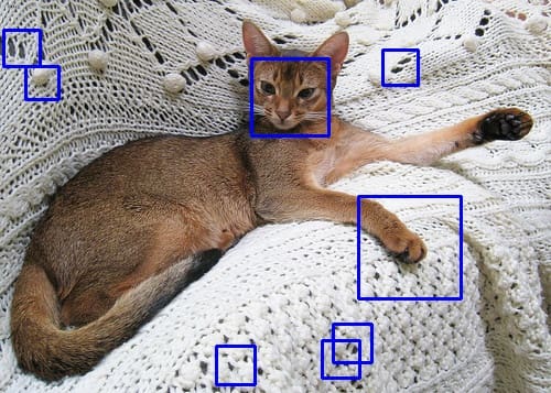
Instance output utilizing the educated Haar cascade object detector
You see some false positives, however the cat’s face has been detected. There are a number of methods to enhance the standard. For instance, the coaching dataset you used above doesn’t use a sq. bounding field, whilst you used a sq. form for coaching and detection. Adjusting the dataset might enhance. Equally, the opposite parameters you used on the coaching command line additionally have an effect on the consequence. Nonetheless, you have to be conscious that Haar cascade detector may be very quick however the extra phases you utilize, the slower it will likely be.
Additional Studying
This part supplies extra assets on the subject if you wish to go deeper.
Books
Web sites
Abstract
On this put up, you discovered the way to practice a Haar cascade object detector in OpenCV. Specifically, you discovered:
Find out how to put together information for the Haar cascade coaching
Find out how to run the coaching course of within the command line
Find out how to use OpenCV 3.x to coach the detector and use the educated mannequin in OpenCV 4.x
Get Began on Machine Studying in OpenCV!
Learn to use machine studying methods in picture processing tasks
…utilizing OpenCV in superior methods and work past pixels
Uncover how in my new E book:Machine Learing in OpenCV
It supplies self-study tutorials with all working code in Python to show you from a novice to skilled. It equips you withlogistic regression, random forest, SVM, k-means clustering, neural networks,
and rather more…all utilizing the machine studying module in OpenCV
Kick-start your deep studying journey with hands-on workouts
See What’s Inside


")

")

")


